F. Results and Graphics

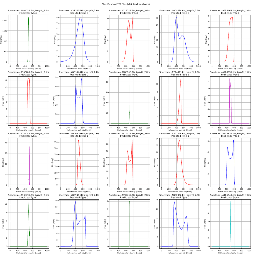
This work proposes a framework for the classification of neutral hydrogen (HI) spectral profiles using Machine Learning (ML) techniques. Unsupervised methodologies and Convolutional Neural Networks (CNN) were applied to analyze 318 profiles from the CIG catalog and 30,780 profiles from the ALFALFA survey. The process included data preprocessing using the Busyfit package, iterative fitting with polynomial, Gaussian, and Lorentzian models, and various classification techniques like KNN, SVM, and Random Forest. Classification was enhanced by adding a 2D dimension to the profiles to study asymmetry. The methodology could be applied to future studies, such as those involving the SKA.

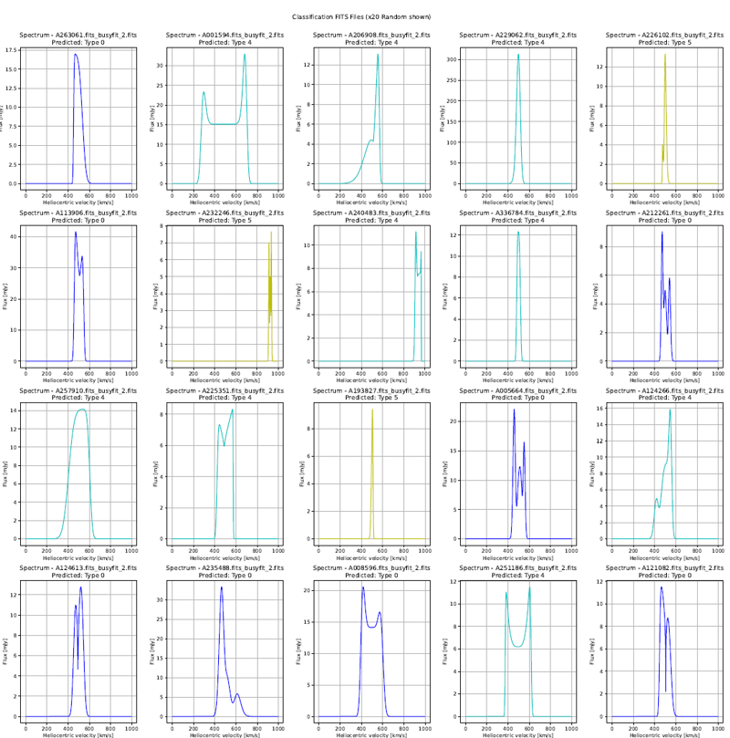
Classification Results + Original Filtered Data

Classification Results

---

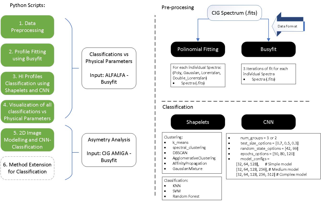
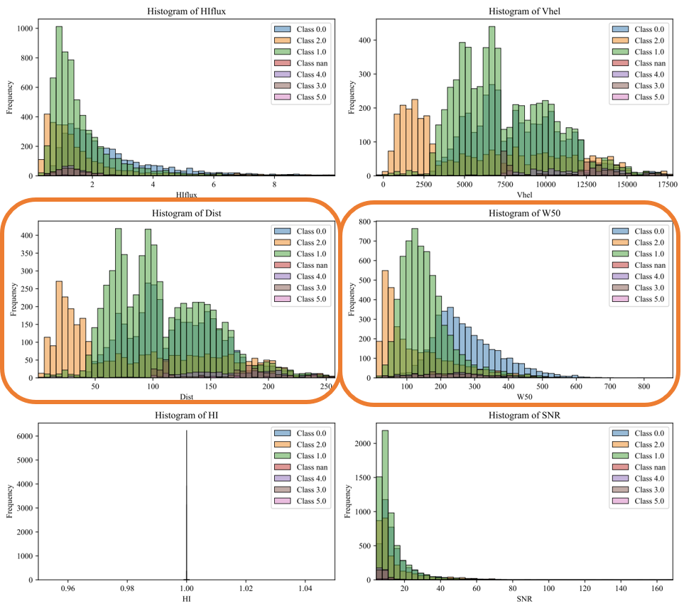
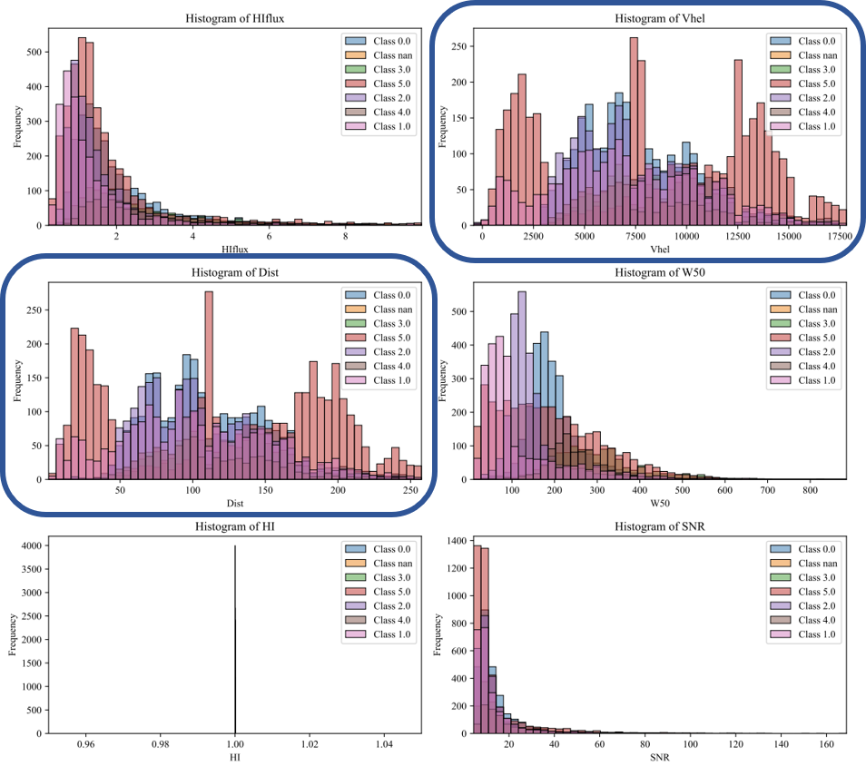
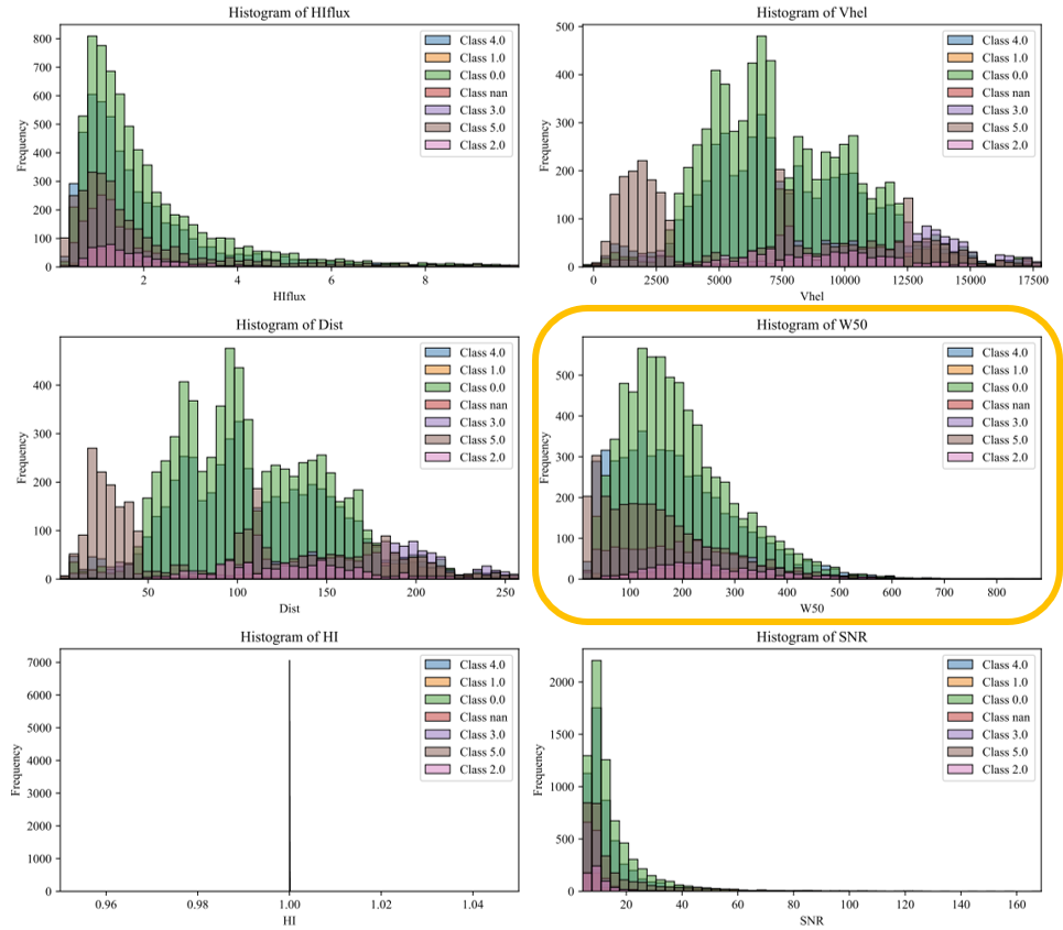
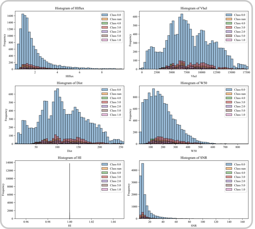
Classifications vs Physical Parameters | Input: ALFALFA - Busyfit

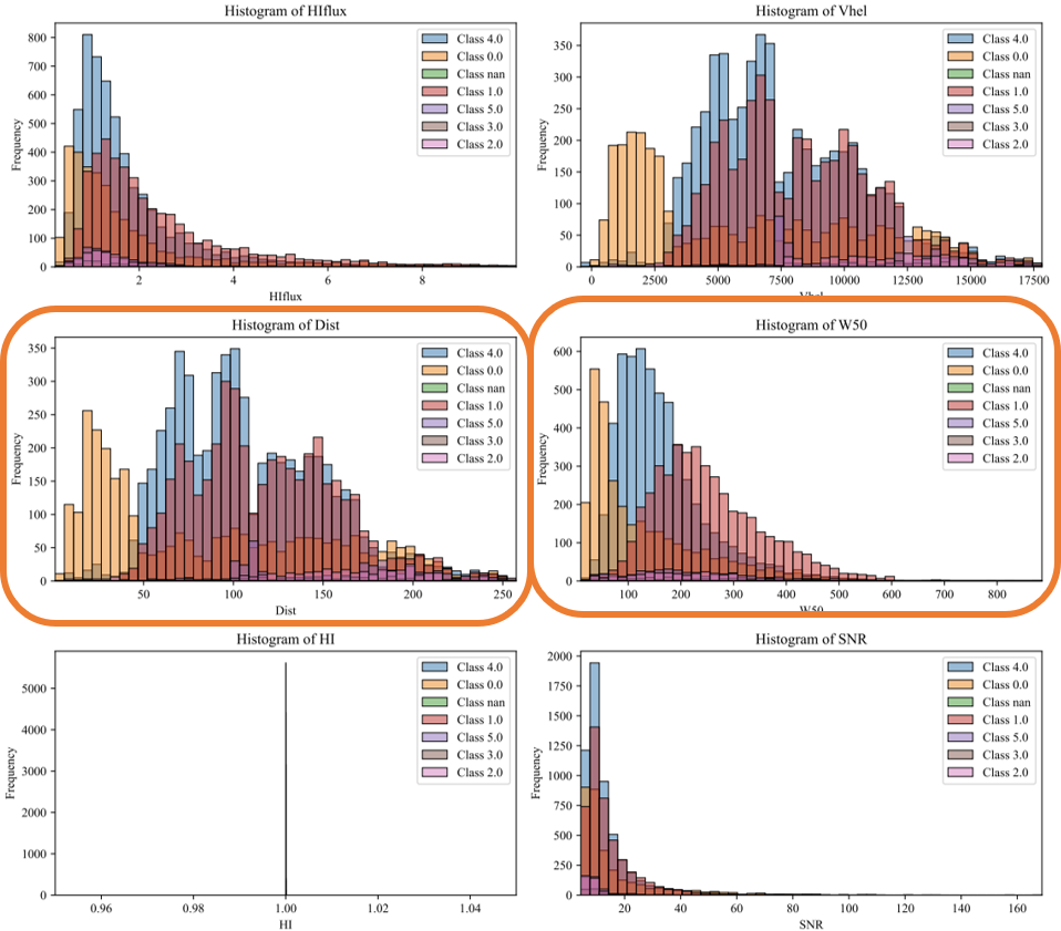
A. Classification: Random_Forest_Shapelets, Clustering Method: spectral_clustering.

• The classification suggest that Class 0,1,2 follows the Width of Spectrum

• Class 2 & Class 1 seems to differentiate from 50 Mpc

B. Classification: KNN_Regular_Shapelets, Clustering Method: spectral_clustering. - The classification suggest that Class 0,1,2 follows the Width of Spectrum - Class 2 & Class 1 seems to differentiate from 50 Mpc

C. Classification: KNN_Regular_Shapelets, Clustering Method: AffinityPropagation. - Class 2 seems to reach peaks by Ranges of Vhel & Dist - There is an aglomeration of classification from 50 to 200 Mpc

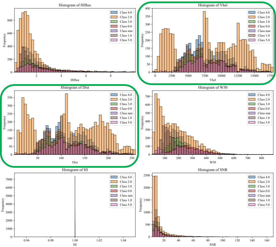
D. Classification: SVM_Shapelets, Clustering Method: k_means. - Class 2 seems to reach peaks by Ranges of Vhel & Dist - There is an aglomeration of classification from 50 to 200 Mpc

E. Classification: Random_Forest_Shapelets, Clustering Method: k_means - Class 2 seems to reach peaks by Ranges of Vhel & Dist - There is an aglomeration of classification from 50 to 275 Mpc

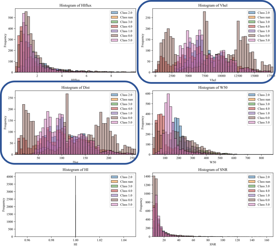
F. Classification: SVM_Shapelets, Clustering Method: AffinityPropagation - Class 0,2,3,4,5 seems to be ordered by frequency (counts) in a similar range of W50

G. Classification: Random_Forest_Shapelets, Clustering Method: DBSCAN - General Application of DBSCAN does not develops a good clustering/classification

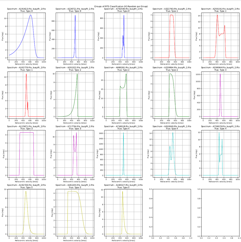
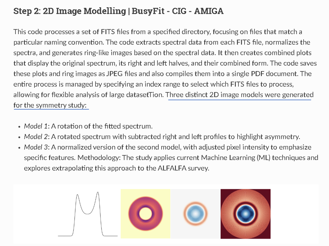
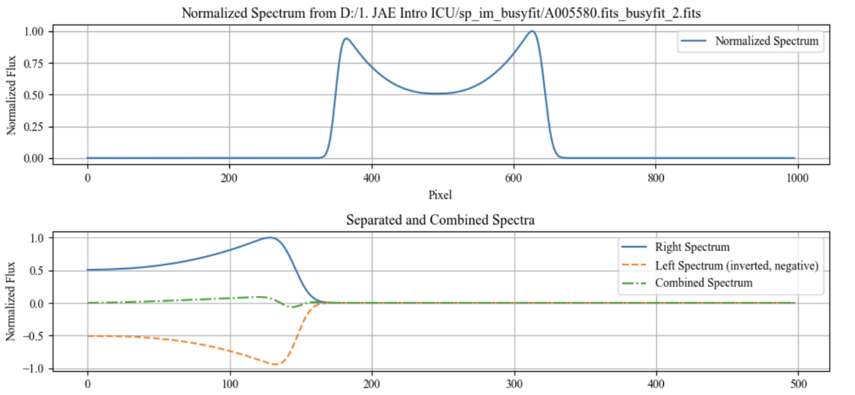
Asymetry Analysis | Input: CIG AMIGA - Busyfit

Asymetry analysis:

Differentiate iterations by changes in (time of each classification: 1.13 hrs, 41 iteration in total):

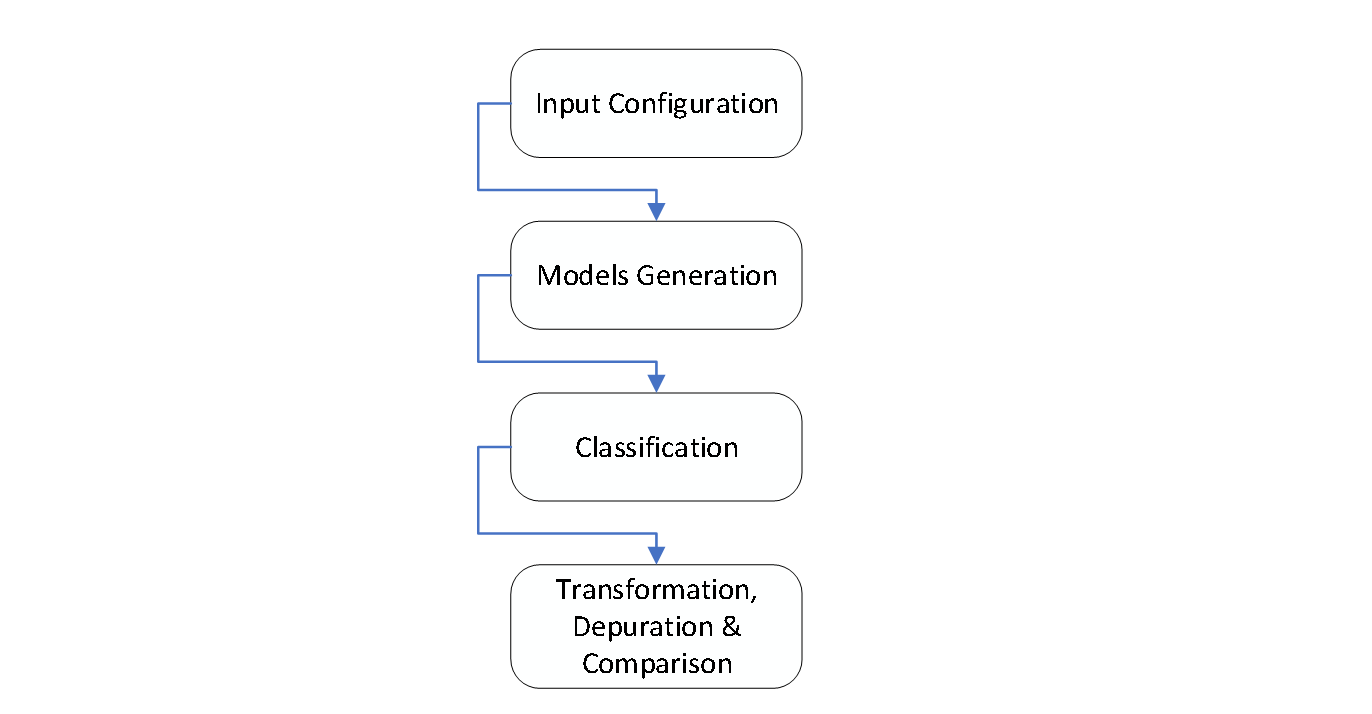
Input configuration

• Selection of 2D Image Model
• Quantity of Data (318 Spec, but Class 0, 1 & 3 are nor balanced)
• Crop of Image (1quarter)
• Reduction of 3 Class into to 2 (0 & 2, balanced and unbalanced)

Classification & Clustering:

Multiple CNN classification are made with iterations usinf the classification model:

    file_suffix = "_rot_im_2.jpeg"
    ...
    num_groups = 3
    test_size_options = [0.7, 0.5, 0.3]
    random_state_options = [42, 99]
    epochs_options = [50, 80, 120]
    model_configs = 
        [32, 64, 128],      # Simple model
        [32, 64, 128, 256], # Medium model
        [32, 64, 128, 256, 512] # Complex model

As Output it is obtained:

Best configuration: Model Config: [32, 64, 128], Test Size: 0.3, Random State: 42, Epochs: 80, Success Rate: 0.6333333333333333

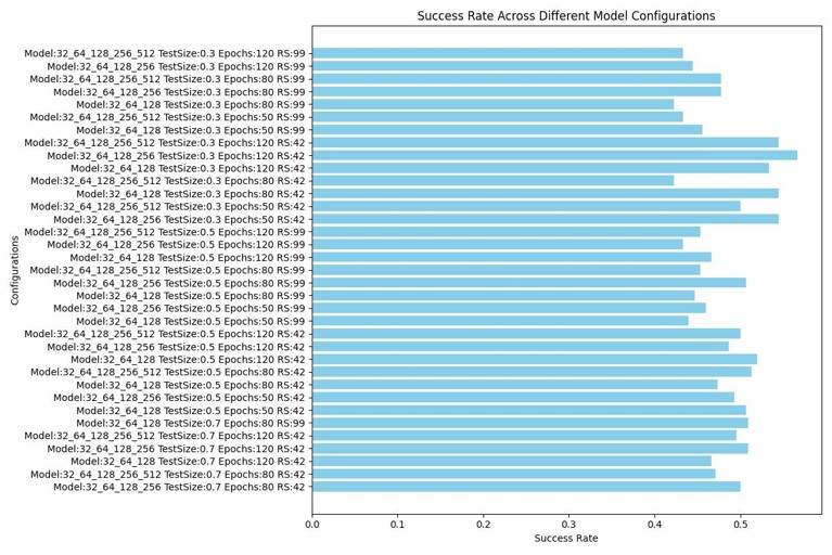
Conclusions:

• Best Success Rates produced with “im_rot_2.fits”.
• CNN Differentiate between colors and shapes according to model classification.
• 2D Image model increase success rate in a 13% in comparison to regular CNN 1D classification and Shapelets Transformations.
• By doing classification with changes in Inputs and Models, theres is a consistent maximum classification rate reaching 63% of Success. It is suggested this is directly related with the size of the sample.
• The methodology generates 54 classifications configuration per iteration, making a depuration and transformation for comparison with an already done classification (D.Espada 2010). In exchange requires computational resources to complete them (1.13 Hrs/per iteration, RAM 16,0 GB – 8 Cores).